Tutorial 1: Approximate MNIST#
This notebook will walk you through the steps required to train a simple CNN on the MNIST dataset while determining the robustness to additive Gaussian noise.
agnapprox already comes with predefined implementations for an MNIST dataset loader as well as LeNet5 which we will use in this tutorial. The next tutorial will show you how to define your own architecture.
%load_ext autoreload
%autoreload 2
from agnapprox.nets import LeNet5
from agnapprox.datamodules import MNIST
CUDA not found, running on CPU
We first set up the datamodule. Downloaded datasets are written to the path pointed to by the environment variable AGNAPPROX_DATA_DIR by default. If the variable is not set, the subdirectory data is created locally.
dm = MNIST(batch_size=128, num_workers=4)
dm.prepare_data()
dm.setup()
Next, we define the model. We can simply instantiate the appropriate agnapprox wrapper without anything else.
model = LeNet5()
Model Training#
Every agnapprox network has four modes in which the network can be trained:
Baseline: Train an FP32 baseline model without quantization, approximation, AGN, etc.
Quantization-aware Training: Apply quantization during the forward pass. Also known as quantization-aware training
Gradient Search: Add Gaussian noise to the output of each target operation. The amount of noise injected in each layer is passed to the optimizer and optimized together with the other network parameters.
Approximate Retraining: Use Lookup tables of approximate multipliers to retrain the network in order to minimize the loss of accuracy when deploying approximate multipliers
Normally, you would train a model in every mode in the order given above (but feel free to experiment with other setups!). agnapprox network instances provide training functions for each mode with some added functionality. The training functions are wrappers around pytorch-lightning’s Trainer() API and extra arguments can be passed to the fit() method if desired.
We will start with a simple FP32 baseline model. The default number of epochs for each stage is defined in the network wrapper file, but it can be overridden by passing epochs= to the training function. Here, we will train for 8 epochs.
model.train_baseline(dm, epochs=8, test=True)
GPU available: False, used: False
TPU available: False, using: 0 TPU cores
IPU available: False, using: 0 IPUs
HPU available: False, using: 0 HPUs
  | Name  | Type   | Params
---------------------------------
0 | model | LeNet5 | 61.9 K
---------------------------------
61.9 K    Trainable params
0         Non-trainable params
61.9 K    Total params
0.248     Total estimated model params size (MB)
/home/elias/agn-approx/.venv/lib/python3.8/site-packages/pytorch_lightning/trainer/trainer.py:653: UserWarning: Detected KeyboardInterrupt, attempting graceful shutdown...
  rank_zero_warn("Detected KeyboardInterrupt, attempting graceful shutdown...")
────────────────────────────────────────────────────────────────────────────────────────────────────────────────────────
       Test metric             DataLoader 0
────────────────────────────────────────────────────────────────────────────────────────────────────────────────────────
      test_acc_top1         0.9850999712944031
        test_loss           0.04709929972887039
────────────────────────────────────────────────────────────────────────────────────────────────────────────────────────
Next, we optimze the model for 8-Bit quantization using the train_quant functions. If you are wondering where the training hyperparameters like optimizer, learning rate, learning rate schedule etc. are coming from: They are also pre-defined in the network’s definition.
model.train_quant(dm)
GPU available: False, used: False
TPU available: False, using: 0 TPU cores
IPU available: False, using: 0 IPUs
HPU available: False, using: 0 HPUs

  | Name  | Type   | Params
---------------------------------
0 | model | LeNet5 | 61.9 K
---------------------------------
61.9 K    Trainable params
0         Non-trainable params
61.9 K    Total params
0.248     Total estimated model params size (MB)
`Trainer.fit` stopped: `max_epochs=1` reached.
Robustness Optimization#
Now comes the exciting part: We train while optimizing the amoung of AGN per layer. By passing verbose=True we get a debug output with the intermediate results after every epoch.
# Set appropriate log level and send to stdout so that logging output shows up in Jupyter
import logging
logging.basicConfig(level=logging.INFO, stream=sys.stdout)

model.train_gradient(dm, lmbd=0.2, initial_noise=0.025)
GPU available: False, used: False
TPU available: False, using: 0 TPU cores
IPU available: False, using: 0 IPUs
HPU available: False, using: 0 HPUs

  | Name  | Type   | Params
---------------------------------
0 | model | LeNet5 | 61.9 K
---------------------------------
61.9 K    Trainable params
0         Non-trainable params
61.9 K    Total params
0.248     Total estimated model params size (MB)
INFO:agnapprox.nets.approxnet:Epoch: 0
INFO:agnapprox.nets.approxnet:Layer: model.conv1.0 | sigma_l: +0.061
INFO:agnapprox.nets.approxnet:Layer: model.conv2.0 | sigma_l: +0.426
INFO:agnapprox.nets.approxnet:Layer: model.linear1 | sigma_l: +0.091
INFO:agnapprox.nets.approxnet:Layer: model.linear2 | sigma_l: +0.051
INFO:agnapprox.nets.approxnet:Layer: model.linear3 | sigma_l: +0.017
INFO:agnapprox.nets.approxnet:Epoch: 1
INFO:agnapprox.nets.approxnet:Layer: model.conv1.0 | sigma_l: +0.051
INFO:agnapprox.nets.approxnet:Layer: model.conv2.0 | sigma_l: +0.500
INFO:agnapprox.nets.approxnet:Layer: model.linear1 | sigma_l: +0.068
INFO:agnapprox.nets.approxnet:Layer: model.linear2 | sigma_l: +0.063
INFO:agnapprox.nets.approxnet:Layer: model.linear3 | sigma_l: +0.003
INFO:agnapprox.nets.approxnet:Epoch: 2
INFO:agnapprox.nets.approxnet:Layer: model.conv1.0 | sigma_l: +0.074
INFO:agnapprox.nets.approxnet:Layer: model.conv2.0 | sigma_l: +0.500
INFO:agnapprox.nets.approxnet:Layer: model.linear1 | sigma_l: +0.093
INFO:agnapprox.nets.approxnet:Layer: model.linear2 | sigma_l: +0.081
INFO:agnapprox.nets.approxnet:Layer: model.linear3 | sigma_l: -0.004
`Trainer.fit` stopped: `max_epochs=3` reached.
Multiplier Assignment#
Finally, we can use this information to assign matching multipliers to each layer. This is done through a helper function that gets passed a list of approximate multipliers, from which the best-matching one is picked for each layer.
Each multiplier in the list should be a dataclass instance that looks like this:
@dataclass
class ApproximateMultiplier
    name: str
    performance_metric: float
    error_map: np.ndarray
For the parameter performance_metric, you can choose any property that you want to minimize across the your neural network. Normally, this would likely be things like power consumption, area usage, etc.
Error Map Construction#
The error_map is a numpy array of shape 256x256, where each entry corresponds to the difference between the accurate and the approximate result for int8 operands:
error_map = np.empty([256,256])

for x in range(-128, 128):
    for y in range(-128, 128):
        error_map[x+128][y+128] = x * y - approx_mult(x, y)
Where approx_mult is some approximate multiplication implementation.
# Import a few helpers and a provider of approximate multipliers
from agnapprox.utils import select_multipliers, deploy_multipliers
from evoapproxlib import EvoApproxLib
import pytorch_lightning as pl

trainer = pl.Trainer()
evo = EvoApproxLib()
target_multipliers = evo.prepare(signed=True)

print(", ".join([tm.name for tm in target_multipliers]))
GPU available: False, used: False
TPU available: False, using: 0 TPU cores
IPU available: False, using: 0 IPUs
HPU available: False, using: 0 HPUs
mul8s_1KR3, mul8s_1KR6, mul8s_1KR8, mul8s_1KRC, mul8s_1KTY, mul8s_1KV8, mul8s_1KVA, mul8s_1KVB, mul8s_1KVL, mul8s_1KX2, mul8s_1L1G, mul8s_1L2D, mul8s_1L2H
# Match multipliers to layers
res = select_multipliers(
    model, dm, target_multipliers, trainer
)
# Deploy selected multipliers to each layer
deploy_multipliers(model, res, evo)
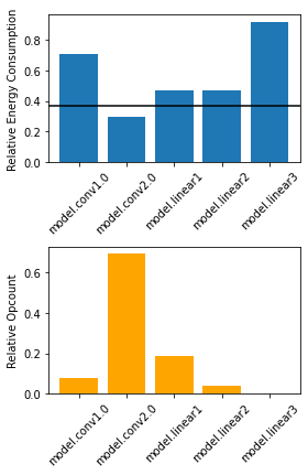
INFO:agnapprox.utils.select_multipliers:Layer: model.conv1.0, Best Match: mul8s_1L2H, Performance: 0.301000, Relative Performance: 0.708235
INFO:agnapprox.utils.select_multipliers:Layer: model.conv2.0, Best Match: mul8s_1L1G, Performance: 0.126000, Relative Performance: 0.296471
INFO:agnapprox.utils.select_multipliers:Layer: model.linear1, Best Match: mul8s_1L2D, Performance: 0.200000, Relative Performance: 0.470588
INFO:agnapprox.utils.select_multipliers:Layer: model.linear2, Best Match: mul8s_1L2D, Performance: 0.200000, Relative Performance: 0.470588
INFO:agnapprox.utils.select_multipliers:Layer: model.linear3, Best Match: mul8s_1KX2, Performance: 0.391000, Relative Performance: 0.920000
If we look at some data, we see that the layer with the most multiplications gets assigned the hardware instance with the lowest energy consumption, while the first and last layers remain relatively accurate.
import matplotlib.pyplot as plt
import numpy as np


x = np.arange(len(res.layers))
multiplier_performance = np.array([l.relative_energy_consumption(res.metric_max) for l in res.layers])
opcounts = np.array([l.relative_opcount(res.opcount) for l in res.layers])
labels = [l.name for l in res.layers]

plt.figure(figsize=(4,6))
plt.subplot(211)
plt.bar(x, multiplier_performance)
plt.xticks(x, labels, rotation=45)
plt.ylabel('Relative Energy Consumption')
plt.axhline(res.relative_energy_consumption, color='black')

plt.subplot(212)
plt.bar(x, opcounts, color='orange')
plt.xticks(x, labels, rotation=45)
plt.ylabel('Relative Opcount')
plt.tight_layout()
plt.show()
Approximate Retraining#
We have selected an approximate multiplier for each layer and deployed them. The last step is to retrain the network while simulating the selected approximate multipliers so that the network learns to compensate for the error.
model.train_approx(dm, test=True)
GPU available: False, used: False
TPU available: False, using: 0 TPU cores
IPU available: False, using: 0 IPUs
HPU available: False, using: 0 HPUs

  | Name  | Type   | Params
---------------------------------
0 | model | LeNet5 | 61.9 K
---------------------------------
61.9 K    Trainable params
0         Non-trainable params
61.9 K    Total params
0.248     Total estimated model params size (MB)
`Trainer.fit` stopped: `max_epochs=5` reached.
────────────────────────────────────────────────────────────────────────────────────────────────────────────────────────
       Test metric             DataLoader 0
────────────────────────────────────────────────────────────────────────────────────────────────────────────────────────
      test_acc_top1         0.9914000034332275
        test_loss           0.02799428068101406
────────────────────────────────────────────────────────────────────────────────────────────────────────────────────────
Uniform approximation#
Finally, we can compare that to a uniform solution where the same approximate multiplier is used across all layers
for n,m in model.noisy_modules:
    m.approx_op.lut = evo.load_lut('mul8s_1L2D')

model.train_approx(dm, test=True)
GPU available: False, used: False
TPU available: False, using: 0 TPU cores
IPU available: False, using: 0 IPUs
HPU available: False, using: 0 HPUs

  | Name  | Type   | Params
---------------------------------
0 | model | LeNet5 | 61.9 K
---------------------------------
61.9 K    Trainable params
0         Non-trainable params
61.9 K    Total params
0.248     Total estimated model params size (MB)
`Trainer.fit` stopped: `max_epochs=5` reached.
────────────────────────────────────────────────────────────────────────────────────────────────────────────────────────
       Test metric             DataLoader 0
────────────────────────────────────────────────────────────────────────────────────────────────────────────────────────
      test_acc_top1         0.9918000102043152
        test_loss          0.025801436975598335
────────────────────────────────────────────────────────────────────────────────────────────────────────────────────────
Depending on your initialization, the uniform solution might sometimes end up having a slightly better accuracy compared to the heterogeneous solution. This is because MNIST is an extremely simple problem and this notebook does not used hyperparameters that are particularly well-tuned.